Inflation Outlook: Likely Worse Than Expected

Though money supply has been growing rapidly over the period since the Great Recession in 2008, not much of it has been put to productive use through credit extension to finance economic activity. Instead, the Federal Reserve Bank (Fed) has incentivized the banking system to hold excess reserves at the Fed. The Fed’s policy was to provide a safe yield – the so named IOER, or interest on excess reserves – if reserves were parked in an account at the Fed. Required reserves.
Bank reserves zoomed to $2.8 trillion from $45 billion in 2010. Even required reserves, though a small portion of total reserves, increased from $43 billion to $208 billion by early 2020. Following the declaration of a Covid-19 pandemic, reserve requirements were dropped to zero on March 26, 2020. So, up until March last year, there has been no need by banks to take market risk when the Fed provided a safe return. That largely worked to sterilize the growth in money supply so that little new credit was extended to finance economic activity.
That is about to change. Interest rates are rising, suggesting greater opportunity costs (forgone returns) for not putting the money to work throughout the economy. It isn’t just banks that will face greater incentives. As a consequence, nominal economic activity will be stimulated and consumer price inflation is likely to reach higher rates. The implication is for increased monetary velocity that will push up nominal GDP and with it likely push consumer prices to 3.5% or more in the next few years. Our forecast is a full percentage point higher than the forecast embedded in the TIPS five-year forward inflation rate. While the Fed believes it has the tools to control price inflation, it has indicated that they are determined not to let it get out of control. To combat accelerating price inflation it will likely put them in a bind as they are forced to raise short-term interest rates. That will likely lead to adverse consequences for the stock market and real economic growth.
AIER’s Past Research on Inflation
AIER has a long interest in the causes of inflation. The Institute believed in the classical view that price inflation is caused by too much money chasing too few goods. In other words, inflation of prices begins with inflation of the money supply. This theoretical view has not fared well in recent decades, because nominal GDP growth and inflation did not reflect the growth in money. Something else was absorbing the growth in money. Price inflation was trending downward so rapidly it almost reached the point where many feared deflation was just around the corner.
What constitutes money and the policies, actions and economic circumstances that artfully have led to the sterilization of the growth in high-powered money issued by the Fed have reduced conventional analysis to a state of confusion.
At AIER, in 1933, founder E.C. Harwood developed a unique indicator of inflationary pressure by distinguishing between the types of money and credit created by the banking system. He did so determining and differentiating between sound and unsound sources of money and credit. Unsound sources of money and credit were considered inflationary.
Harwood determined that, under the gold standard and early 20th century banking practices, sound (i.e. “noninflationary”) money consisted of bank and Federal Reserve notes and checking and savings balances backed by reserves of gold, bank capital, and deposits. Sound credit was that credit representing short-term loans for goods coming to market. It also included loans based upon deposited savings. Unsound, (i.e. “inflationary”) credit, according to Harwood, was that created by banks for other types of loans that are not backed by deposits, gold or capital reserves (See AIER, E.C. Harwood, Causes and Control of the Business Cycle, 1932).
What came to be known as the Harwood Index of Inflating sought to measure the growth of excess purchasing media; that is, money and credit in circulation originating from inflationary sources. Considerable research effort was expended to gather data from the Federal Reserve system. The Index was successfully used to forecast business cycle activity for a number of decades, until in the 1970s the Fed ceased publishing the useful information that made calculations possible. Nonetheless, at its base, his achievement was to substantiate that price inflation, no matter how it manifests itself in the economy, begins with monetary inflation.
The Meaning of Inflation
In the everyday world, the economic measurement of inflation is confusing; it is a many-headed hydra. The word has been used to refer to inflating the measurement of the economy in nominal terms – GDP; inflating the price of consumer goods and services – CPI; inflating the prices of assets, such as the stock market, real estate, art, gold and other collectibles; deflating the value of the currency; monetary inflating, i.e. the process of creating money through a centralized source such as the Federal Reserve; or all of the above. From a root cause point of view E. C. Harwood chose to focus on the measurement of excessive money growth.
As an economic behavioral concept, the common sense understanding of the causes and effects of price inflation is another many-headed serpent. There are different theories for the causes of price inflation. For example: rapid growth in money supply; rapid growth in income causing rapid growth in demand relative to supply; rapid increase in the cost of labor relative to productivity gains.
The effects of price inflation are fairly clear – the impoverishment of the consumer and increased maldistribution of wealth, favoring those who own assets over those who do not. Consumers are impoverished because a dollar of disposable income will not go as far. Were disposable income to rise as rapidly as inflation there would be an offset. That is usually not the case during periods of rising price inflation.
Price Inflation and Its Relation to Money
The causes and the measurement of inflation have inspired many theories beside that of E.C. Harwood’s pioneering work in 1932. It continues to be a battleground of theory and philosophy: Marxist versus Austrian theory; Chicago monetarist versus London Keynesian theory. None have achieved universal acceptance among economists.
For the purposes of this paper, we take the classical view of money and its relation to inflation. Money is both a medium of exchange and a commodity. As such, the price of money and its quantity availability is governed by supply and demand schedules. The price of immediately available money is the spot rate, a risk-free interest rate, that is close to nil. The longer the term of holding, which means the less the liquidity (immediacy of availability), the higher the price.
Long-term interest rates reflect the returns that can be earned from alternative uses of money. Long-term interest rates measure the opportunity cost of money for a particular future period of time, i.e. maturity. Other examples of opportunity cost would be the return the money could earn if it were put to work in a real investment. The opportunity cost provides a return to the lender of funds that covers business and inflation risks and provides enough for a real rate of return. The borrower of funds puts the money to work at his cost plus a profit margin to cover his risks.
As the difference between the longer-term rates and the spot rate increase there is an incentive to more aggressively seek alternative investments to put money to work instead of leaving it idle and earning zero interest.
In a free market system, excesses in the monetary system ultimately will result in a general rise in the price level. However, price inflation can materialize in various places in the economy. It can spring up in any sector of economic activity including consumer goods and services, financial markets, other assets and collectibles. Where it springs up depends on the opportunity costs and regulatory incentives that may favor certain asset classes relative to others.
Price inflation can also arise from supply shocks, interruptions of availability that create shortages. However, this cause usually only results in short-term pressures on prices.
In recent times, though money and potential extensions of credit to finance consumption have been in abundance, they have largely lain idle as the opportunity cost of money has been low. That is in the process of changing as opportunity costs rise. Adding to the darkening inflation picture is the fact that demand for goods and services is coming back quickly in the face of fiscal stimulus and supply destruction, particularly in the service sector, due to Government policies related to Covid-19.
In a fiat paper monetary system, consumer price inflation will reduce purchasing power. Asset price inflation will also arise and may appear to be a hedge, but only for those more fortunate who have significant savings that are in the right appreciating assets. Those less fortunate fall behind.
No matter the causes of the coming inflation, the inevitable effect will be to impoverish on both an absolute and relative basis.
A Quantitative Look – Money and Economic Activity
Currently there are three definitions of money supply provided by the Fed: M1, M2 and MZM. M1 is a narrow definition consisting of cash and checking deposits and M2, a broader concept that includes M1 plus savings deposits, money market securities, mutual funds, and other time deposits. In magnitude, today MZM is greater than M1 or M2. MZM is M2 less time deposits plus institutional money market funds. The latter are often referred to as sweep accounts and a liquid because they can be wired in and out on a day-to-day basis. Specifically MZM is designed to only include forms of money that bear little or no interest and have immediate liquidity. Today they are vastly larger than retail time deposits. MZM went from being less than M2 prior to 2001, to being greater today. In January, 2021 MZM was $21.97 trillion and M2 was $19.39 trillion.
For our analytical purposes MZM is the preferred concept.
All three concepts are depicted in Chart 1. The scale is logarithmic to better display growth rates of the respective measures. MZM is highlighted as a solid line.
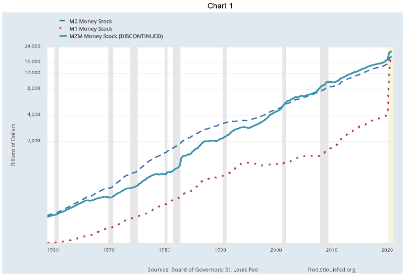
The overall growth patterns are similar, but MZM has clearly grown more quickly than the other measures. Of particular note is the remarkable jump in 2020 of all three measures, especially M1. This sharp move up reflected the Fed’s effort to flood the financial system with credit on very easy terms during the pandemic-induced collapse of economic activity.
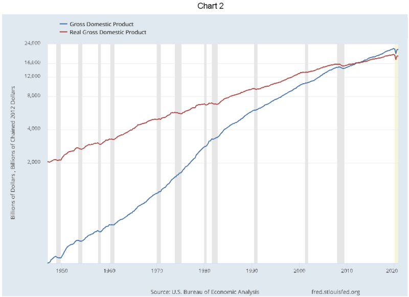
Chart 2 lays out the history of Gross Domestic Production (GDP) in nominal and real terms. GDP measures the total value of all goods and services produced for sale in the final market.
The constant dollar GDP is the nominal value deflated by a price index that is set equal to 100 in 2012, which explains why prior to 2012 the real values were greater than the nominal values. The more rapidly rising slope for nominal GDP reflects more rapid inflation than real growth. Following the 1981-82 recession the reverse was true – inflation was lower than real growth. (The inflation rate history is shown separately in Chart 5.)
Calculating Velocity of Money
The velocity of money is a concept that measures the turnover of the money supply in the process of generating economic activity; that is the number of times money changes hands in the course of a year. Some activities involve very rapid turnover such as retail commerce. Other activities involve long intervals between transactions such as cash kept in reserve for a rainy day that can sit for years under the proverbial mattress or sitting in an idle balance in a checking account beyond what would normally be held as a precautionary balance.
In this study we measure velocity by dividing nominal GDP by the quantity of money, MZM, as defined earlier.
The concept of the velocity of money was carefully defined and researched by Milton Friedman and others at the University of Chicago in the 1950s. His seminal research, published in 1956 was entitled Studies in the Quantity Theory of Money. His concern was to understand the determinants of the demand for money, its effects on the aggregate economy, and the velocity of turnover of money. At that time he used a measure of money, then known as M3, which today is no longer available from the Fed. Friedman famously concluded that “inflation is always and everywhere a monetary phenomenon.”
For our purposes MZM is a superior concept that was not available at the time of Friedman’s research. This measure only includes forms of money that are immediately available for spending and bear little or no interest (yield) – a feature that is important to understanding why the velocity of money may be sensitive to the level of interest rates.
Friedman presented a simplified framework of analysis that he referred to as the “equation of exchange”, that is: Money(M) times the Turnover of Money(V) equals the value of an economy’s output (GDP), or:
(1) M x V = GDP
The value of the economy’s output is itself a combination of the quantity of goods and services produced, that is, real GDP (or Q), and the prices of those outputs (P), or:
- GDP = Q x P
By simple substitution of (2) into (1), you have:
(3) M x V = Q x P
Solving for velocity of money (V), one obtains:
- V = (Q x P)/M
No doubt this “equation of exchange” is an oversimplification of the relationship between money and economic activity for several reasons:
- The derivation of V is simply an algebraic manipulation. There is no implication of a direction of causality or if there even is causality. These equations are simply identities. They have no behavioral content.
- Not all money in circulation derives from activity associated with wages, rent, profits, investment returns, and transfer payments from the government, as defined in the National Income and Product Accounts (NIPA) of the US.
- Nor is all money expended in the economy only on goods and services transacted in the final markets (GDP as defined by NIPA).
A simple way to understand why it is said that these are not behavioral equations, which suggest causality, is to consider equation (3). On the face of it, it is not clear that if M were to increase that it would lead to an increase in Q or P or both changing proportionately. Alternatively, V might adjust proportionately downward. In fact nothing in the equation prevents all measurements from changing appropriately and still satisfy the equation at a new higher value of M.
The University of Chicago monetarists did argue that the demand for holding money was driven by the alternatives to holding money; that is, the returns on bonds, equities, collectibles, even human capital. Friedman even allowed for a “portmanteau variable” that included considerations such as payment practices and the tastes and preferences of individuals and institutions.
Velocity of Money Tells a Story
Velocity was relatively constant during the era when Friedman did his basic research. Consequently there was not much empirical work to identify and quantify the factors that might affect velocity. In fact, he would argue that cyclically adjusted, one could assume a constant velocity.
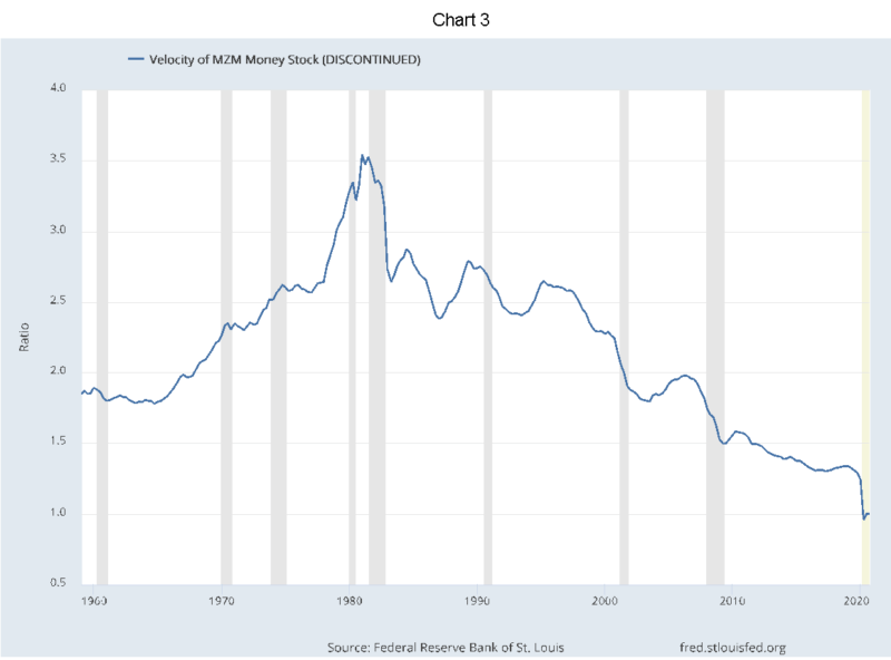
In more recent decades, as shown in Chart 3, calculating money velocity has become very volatile. This has led to great consternation. The turnover of money increased rapidly from just below 2x in the 1960s to 3.5x by 1980-81. Thereafter, velocity fell fairly steadily, reaching 1x in 2020 through the opening months of 2021.
Could one consider the velocity of money to be a function of other variables, such as the interest rate term structure (interest rate with different maturities) , where interest rates are understood to be revealed opportunity costs associated with putting money to work through real investments? In other words, in functional form:
(5) V = f (i1, i2, i3, … )
The recent forty-year secular decline in the velocity of money has astonished many financial economists. From a purely theoretical point of view this was hard to understand. Many Keynesians believed we were surely headed for price deflation (a negative inflation rate). This unique situation would surely be the consequence of a “liquidity trap;” that is, a condition where everyone believes they should hold cash for fear of greater deflation down the road, negative interest rates and crisis of an undefined nature.
Though V, the velocity of money is a calculated number – derived by algebra – does it necessarily follow that it is not influenced by independent forces? We argue that it does and show a functional specification in equation (5) above that V is related to interest rates.
One explanation why velocity continues to decline in the face of increasing money supply is that there are poor or no attractive opportunities in the real economy for putting the money at risk for a period of time. The money obviously has been put to work, but elsewhere outside the productive economy as measured by GDP. When there are attractive investment alternatives, money will be used more intensively – i.e., producing more GDP activity – therefore money velocity with respect to GDP will rise. Money will not be left idle for long.
Conversely, if the opportunity costs are low, that is there are no attractive, risk adjusted returns, that can be earned from investing and surrendering immediate liquidity of the money, then economic activity will slow and the velocity of money will decline.
A flat yield curve is certainly indicative of an environment where there are poor risk-adjusted opportunities available. Not only are yields low, but putting money out at term would expose an investor to substantial principal risk if interest rates rose (duration risk). In reflection of poor financial market opportunities, it is reasonable to conclude that investments in the real economy must be similarly poor as well. One must be a reflection of the other. Therefore, the yield curve is revealing and can be taken as a proxy for the opportunity costs in the real economy.
Unless you were an entrepreneur, it was only through recent financial innovations that the average citizen had access to venture capital or private equity deals. In fact, most investment opportunities that came to market in the form of an IPO came very late in the maturation process of young companies. Most of the early valuation gains were privatized.
For entrepreneurs and small businessmen, there have been massive cross-currents in investment returns. Investments in some industries were sure to lose money as China took over manufacturing sectors that had high labor costs. The US economy has been on a secular shift from manufacturing to service industries. Even in manufacturing, only industries with low unit labor costs had a chance for survival. In the service sector you cannot export the preparation of meals, you cannot export plumbing and electrician jobs. Other than the individual entrepreneur, it is hard to invest in human capital.
To restate, it is reasonable to argue that the risks and returns in the financial markets, as revealed in yield curves for government and corporate issuances, mirror what is available in the real world. This article makes a simplifying assumption. It makes the argument that what is observed in the 10-year US Government Bond interest rate is a good overall surrogate for the opportunity costs available to holders of zero maturity money. If you will, in the words of Friedman, the 10-year rate might be a good proxy for his “portmanteau variable”.
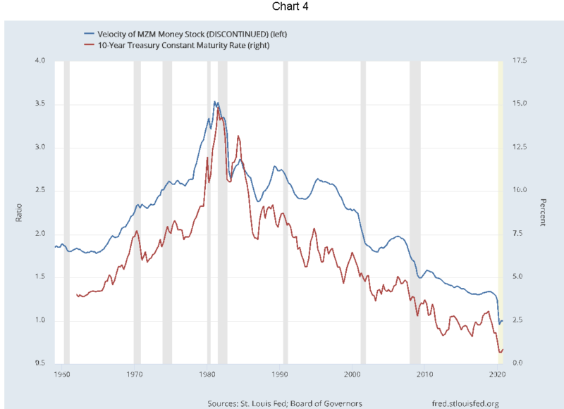
Chart 4 presents an overlay of the 10-year U.S. Treasury interest rate on our calculation of velocity based on MZM.
There is broad synchronization as to movements and timing of the two variables. When the 10-year rate was rising from 1960-1980, velocity rose. When the 10-year rate peaked and began its 40-year descent to below 1%, the velocity of money followed.
In short, money was used more ”intensely,” and turned over more rapidly when there were high opportunity costs, and less intensely when rates were low. When interest rates were nil, the man in the street couldn’t be bothered to move new money into an interest-bearing account or a CD, to be tied to maturity date, with penalties for early redemption. Money was left as an idle checking account balance. For banks, there was no need to take any entrepreneurial risk. It was better to leave excess reserves on deposit with the Fed, and earn the IOER rate. In 2016 it was 0.5% and in 2018 through late 2019 it was over 2.0%. Currently, the rate sits at 0.1%.
The Velocity and Inflation Outlook
The situation is changing. In the last few weeks the 10-year has moved up, touching 2%. The latest CPI numbers are suggesting a quickening of the inflation rate to 2.5%. The TIPS break-even rate also suggests an expectation of 2.5%. Even the Fed has indicated they would tolerate allowing the inflation rate run above the 2% target for a while.
If our hypothesis is correct, the rise in the 10-year Treasury rate will be a precursor to an increase in the velocity of money. Given the huge amount of monetary expansion in the past year this will likely lead to more rapid growth in nominal GDP. With the continuing outlook for bottlenecks and capacity constraints once we reach the summer months, which will limit further rapid growth in real GDP, this is likely to lead to higher price inflation rates.
Another consideration is the ending of one source of price deflation for consumer goods. Since the explosion in internet-based buying, for over 20 years the consumer has benefited enormously from better choices, better service convenience and from lower prices. Retailers have competed to either win business on the internet or keep customers happy in local markets. This has also led to efficiency gains in retailing to stave off collapsing margins from lowering prices. This “wealth” enhancer to the consumers’ income is running its course.
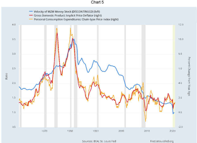
Chart 5 illustrates the path of inflation for the past 80 years, as measured by the price deflator for GDP and the deflator for Personal Consumption Expenditures, in comparison with the velocity of money.
From the graphical relationship, I foresee a high probability that velocity will move back to the 1.5x to 2.0x levels. Were that to occur, consumer price inflation could readily rise to the 3.5-4.0% range. That is a full percentage point above the market’s current forecast as derived from the 5-year forward TIPS breakeven calculation. Some of the more aggressive, return-seeking money could also find its way into equity markets and other assets.
The Fed has painted itself into a box, because if inflation/velocity does heat up beyond what the Fed or markets can tolerate, given that they have been comfortable with somewhat higher long-term rates, the Fed’s only weapon to slow inflation down would be to slow down the economy. Its strongest weapon would be to threaten to push up the short-term rate and invert the yield curve.
The other way would be to significantly slow or reduce money supply. No matter what policy tools would be invoked by the Fed to slow down the inflation monster they have unleashed, the result will be very painful for financial markets.
A Word of Homage and Apology
The pioneering work on understanding the causes of price inflation and the work to create the Harwood Index of Inflating began with the Colonel himself. Over the years, a cadre of researchers, most importantly including: Lawrence Pratt, Ernest Welker and George Machen, pushed the research envelope deeper and further. They eschewed attempts at analyzing velocity as an independent phenomenon. To them, increases in the apparent turnover of money just meant the money was going elsewhere than the production of goods. Their collective concern was to construct a measure that would allow them to sound the alarm when the inflation of money would lead to price inflation of a general nature; that is when it exceeded the production of goods. That was the purpose of the Harwood Index of Inflating. Unfortunately, the viability of continuing their work was cut short by the Federal Reserve’s ending the publication of the necessary data.
Gregory van Kipnis