Take the Government Out of GDP 

With the release of the 2024 Q1 Gross Domestic Product (GDP) data by the Bureau of Economic Analysis, the question of economic growth is on many minds. Real GDP growth slowed to an increase of 1.6 percent from a year ago, lagging well behind the 2.4 percent projection. The BEA commented that the increase is due to “consumer spending, residential fixed investment, nonresidential fixed investment, and state and local government spending that were partly offset by a decrease in private inventory investment” as well as an increase in imports. It is important to note here that the increase in state and local government spending came from an increase in government employee compensation, meaning taxpayers are getting the same government services as last year at a higher cost. 

The nominal GDP equation used by the Bureau of Economic Analysis (BEA) goes as follows: 

Y = C + I + G + NX 

Where Y is GDP or output, C is gross private consumption, I is gross private domestic investment, G is government consumption expenditures and gross investment, and NX is net exports. A common mistake, however, is that GDP gets treated as a simple accounting identity, whereby any increase on the right-hand side of the ledger must mean an increase in nominal output. That is not necessarily the case.  

This analysis aims to look at how the economy is performing without government spending muddying the water. Our aim is to examine the “Gross Domestic Private Product” (GDP excluding government purchases) based on the work of economists such as Robert Higgs, Ryan McMaken, and Matthew Mitchell using updated data from the BEA. 

GDP vs GDPP: Examining the Data  

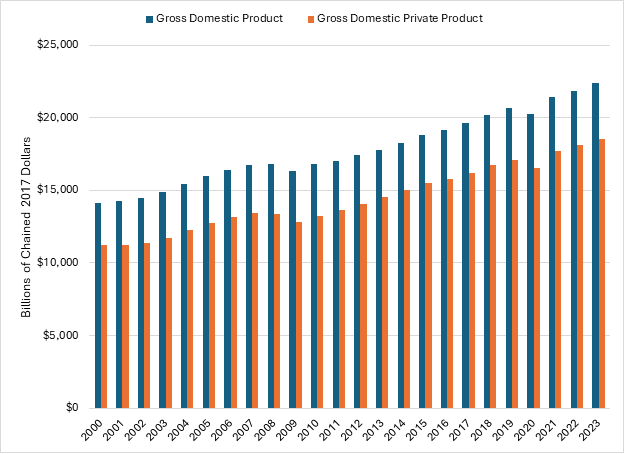
We utilize the data from the BEA website, specifically from the “National Income and Product Accounts” table, in addition to Table 1.1.6 (Real Gross Domestic Product, Billions of Chained 2017 Dollars). To calculate GDPP, we subtract the G  (“Government consumption expenditures and gross investment”) variable from total GDP. Note that G does not include transfer payments, such as Social Security (because Social Security or Unemployment Insurance consumption is counted towards private spending). While the average percentage of G is 25.7 percent for 1950-2023, 28.8 percent for 1950-1999, and 19.2 percent for 2000-2023, total government spending (including transfer payments) as a percentage of GDP is much higher than the variable G. This also does not consider the impact of government debt, which generates a significant level of drag on economic growth. 

In previous analyses, the BEA provided inflation-adjusted numbers in chained 2009 dollars. Starting in 2018, the BEA replaced real GDP estimates in chained 2009 dollars with real GDP in chained 2017 dollars. While the BEA did not provide specific reasons for why they chose 2017 as the new base year for chained dollars, typically such adjustments are made for changes in the relative importance of certain goods and services (weighting), new data methodologies, and/or the diminishing relevance of legacy data. Despite the change in base year, however, we see similar results to the analysis provided by McMacken in 2017 using chained 2009 dollars. Like Higgs and McMacken, we use BEA Table 1.1.6. 

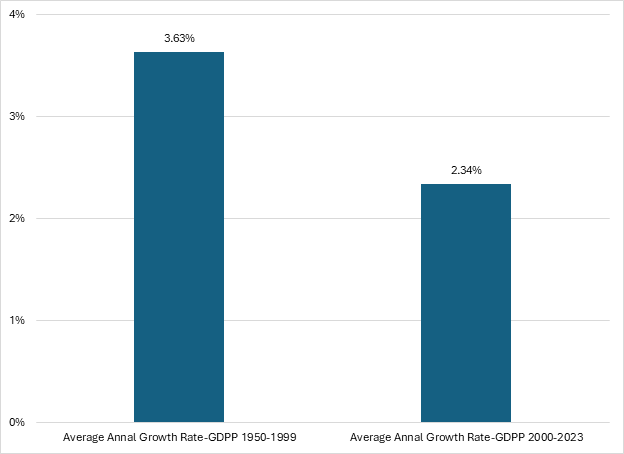
McMaken’s findings in 2017 still hold true today: gross domestic private product growth has slumped. When comparing the average annual growth rate before and after 2000, we see a slump in the average annual growth rate. The figure below shows that the average annual growth rate of GDPP prior to 2000 was 3.63 percent while the post-2000 average was 2.34 percent. While not the stark 50 percent difference shown in McMaken’s analysis (due to data and methodological updates), GDPP has still been growing 35 percent slower per year since the start of the new millennium. 

In Mitchell’s 2010 paper, he also compares these growth rates to the growth rates of the US government. Those charts have been recreated below, covering the same period as the figure above. The average annual growth rates are calculated based on the chained 2017-dollar amounts. (Federal totals include both defense and nondefense spending.) 

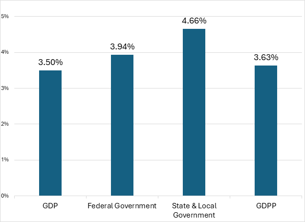
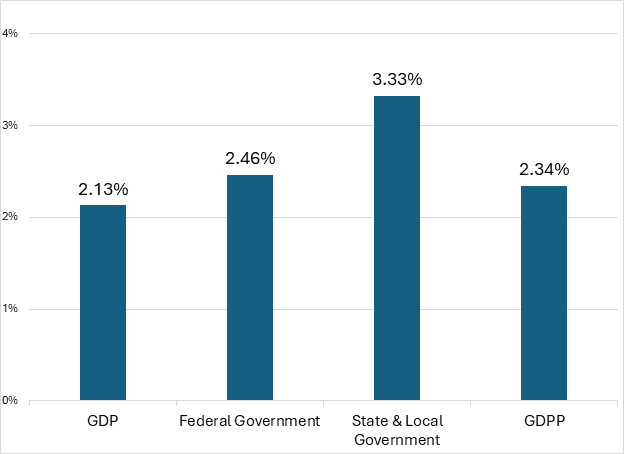
Note that in both time periods government consumption expenditures and gross investment have consistently outpaced private sector growth. State and local governments in particular have outpaced private sector growth. Mitchell notes, and we concur, that the increase in federal transfers has played a direct and substantial role in the rapid growth in state and local governments. Although not directly measured in the BEA estimates, these transfers have allowed state and local governments to increase spending in other areas because they can rely on federal transfers to fund a significant portion of their budget. 

As we noted recently, the dependence of US states upon federal funds has increased at an alarming rate. When federal policymakers inevitably make cuts to those state and local transfers, state and local governments are faced with making large, sometimes unexpected tax hikes and spending cuts to fill funding gaps. And while the federal government has states increasingly dependent upon those transfers, it has the power to exert control over state and local policy, using funding to influence policy that effectively generates an end-run on Congress and the legislative process. And when states face fiscal crises for their unsustainable budget policies, gross domestic private product suffers. The ensuing debt restructuring process drives families and businesses to flee the states in crisis, not only shrinking private investment and consumption but giving rise to an increasing number, and level, of taxation. 

GDP vs GDPP Over the Business Cycle  

Also noted by McMaken, the difference between GDP and GDPP helps analyze the business cycle. The figure below shows the year-over-year changes in quarterly GDP and GDPP. 

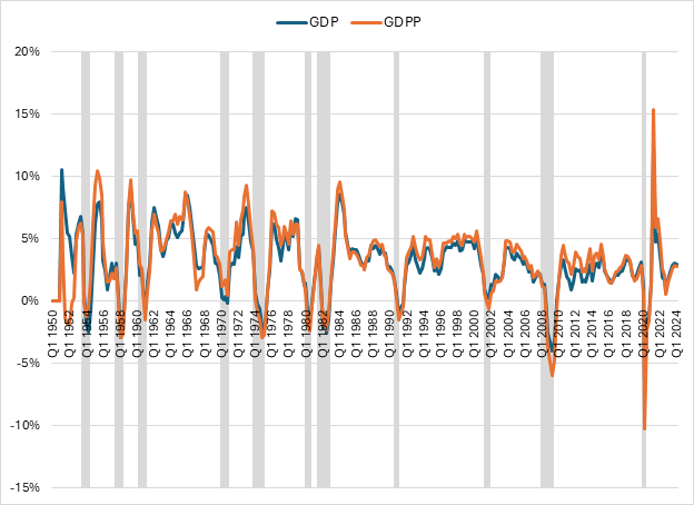
We find that GDPP has year-over-year rates of increase larger than GDP (note again that this excludes government transfer payments). Additionally, GDPP falls more than GDP before recessions. While McMaken remained pessimistic about 2016, we do see a recovery up until the COVID-19 pandemic. The massive increase in 2021 followed by the slump in 2022 is emblematic of government-induced booms from massive government spending and historically expansionary monetary policy programs. 

As mentioned earlier, Q1 2024 GDP estimates fell below projections. As expected, GDPP rose in tandem with GDP. The BEA release states that the decrease in inventory investment (one of the causes of GDP coming in below projections) “reflected decreases in wholesale trade and manufacturing.” The increase in consumer spending was also “partly offset by a decrease in goods,” all contributing to slow GDPP growth. 

Understanding the Cost of Government 

Many people believe that government spending can jump start or boost economic growth. The multiplier effect is a cornerstone of most macroeconomic classes. Yet the embrace of the concept suffers from the classic error of Frederic Bastiat’s Broken Window Fallacy in his equally famous work, What is Seen and What is Not Seen. In it, Bastiat tells a parable of a shopkeeper’s window being broken by his son. Onlookers comfort the store owner, asking, “What would happen to the glassmakers if no window were ever broken?” Sure, the glassmaker is now six francs richer because of the broken window (“What is seen”) but the cost to the shopkeeper is the next highest-valued use of those six francs (“What is not seen”). 

In the private sector wealth is created through voluntary exchange. Two or more parties come together voluntarily and exchange goods or services that of equal or comparable value, benefitting all parties involved. As the late economist Walter Williams put it, “With the rise of capitalism, it became possible to amass great wealth by serving and pleasing one’s fellow man. Capitalists seek to discover what people want and then produce and market it as efficiently as possible as a means to wealth.” 

Government spending, on the other hand, is not peaceful or voluntary exchange, whatever narratives attempt to frame it as such. Tax revenues are harvested from private citizens by means of coercion and extractive measures. If citizens do not comply and pay their taxes, they face fines and jail time. Paying taxes to remain free of incarceration or not face withering financial penalties is hardly indicative of cooperative exchange.  

The economist James Buchanan noted that when governments decide to finance spending by taking on debt, the effects are two-fold. First, private investors purchasing government debt comes at the cost of whatever other projects investors might have otherwise invested in or provided financing for. As Buchanan put it, spending that is funded by debt is “in effect chopping up the apple trees for firewood, thereby reducing the yield of the orchard forever.” Debt-financed spending also shifts tax burdens from present to future generations. While bond investors trust that their loan will be paid back with interest, future generations will bear the cost of the government spending undertaken today. 

With many Americans still feeling the sting of the current tax season, now is an especially pertinent time to reflect on how much money they’ve sent to the government: not only on April 15th, but throughout the year via withholdings, sales taxes, and other takings. Readers should ask themselves, “What could I have done with the money I paid to the government?” And even if one was fortunate enough to receive a refund, all they’ve done is extend an interest-free loan. What might have been done with the monies that were withheld? 

Our goal in examining GDPP is to get readers thinking about the “unseen” costs of government and unraveling how much the US government costs private sector growth. 

Related Articles – Economic Growth, Fiscal Policy, Taxation